Joints Control System

 

Please note Joint Control is still under construction, this section only reflects the status at the moment it was written. Further modification will probably be made and reported later.

The Joint Control System (JCS) uses PID regulators  to control the position. However, I soon realized that many other features were requested in order to tune the joints parameters individually and then on the assembled robot : 

• Bidirectionnal communication with Robot Control Unit (RCU) : I use it in order to log the position / force data and analyse them later. Without data logging, this would be impossible to tune and improve the robot control.
• Possibility to update any parameter used in the control board (gains, offsets, slopes, stiffness, damping ratio,…). For instance, every time the Robot Control Unit  starts, it automatically sends to the JCBs all the latest sets of paramaters. This is very usefull as there is no need to reflash the S/W on the JCB µController every time a parameter is changed.
• Zero angle calibration : check potentiometer position and define related encoder position offset. This calibration procedure is applied every time Joint Control Boards are switched on.

I had to develop 3 variants of the Joint Control System:

• Single Joint position control (z1 and x2 joints)
• Single Joint position with Torque Feedback (y3 and y4 joints)
• Dual Joints position with Torque Feedback (y5 and x6)

Joints Compliance 

JCS Torque feedback can emulate an output shaft with spring and damper. This  gives compliance to the joints, i.e. flexibility when required to accomodate unexpected / unpredictable situations. Compliance is used for example in the following cases :

•  On the lifted leg when walking, to prevent/minimize unbalancing shock when meeting an unexpected obstacle
• On the lifted foot ankle to adapt to the floor condition and avoid unbalacing the walk when landing the foot (especially in uneven terrain). 

Stiffness and damping coefficient can be modified at any moment (Actives modes 65 and 66 – See running modes below).

The emulated model of the output shaft of the joint is as follows :

The emulated spring/damper model produces an actuator position  request (as a function of torque and position derivative) which is then controlled by the PID controller.

Note that under torque, the requested joint position can never be achieved. As stiffness is increasing, position error becomes smaller.

I defined an “infinite” stiffness mode when  setting Ks to 255. 

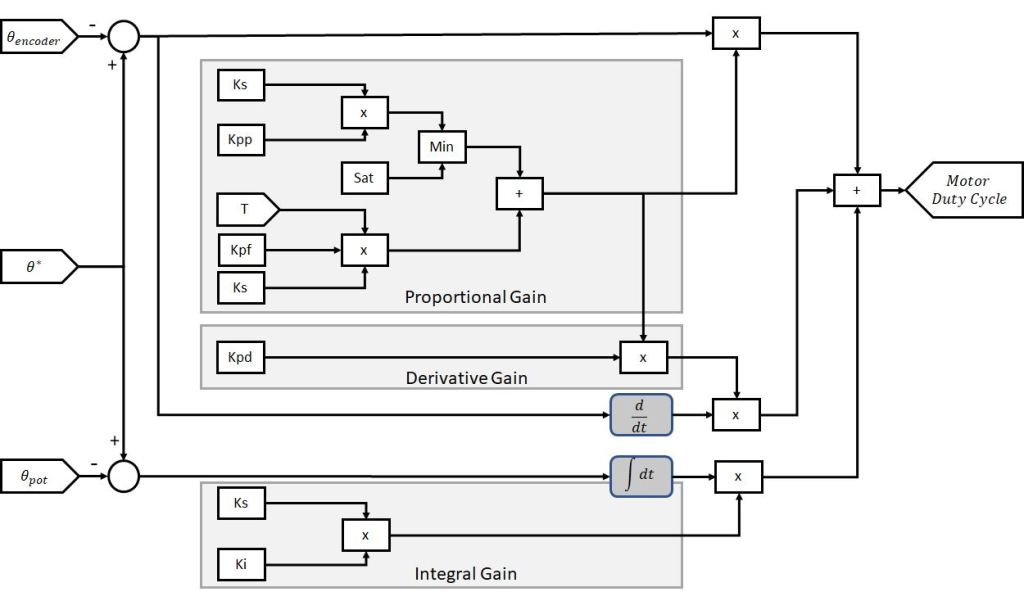
PID Position Control 

The PID controller uses encoder feedback position for  Proportional and derivative control and Potentiometer for Integral control. 

A gain proportional to Torque is added to Proportional and derivative gains (tuned by Kpf). 

All PID gains are made proportional to Spring Stiffness up to a saturation value (defined with gain tuned with infinite stiffness).

Kpp and Kpf set proportional gain, Kpp is multiplied to Ks and Kpf is multiplied to Ks and |Torque|.

Kpd multiplies proportional gain to set derivative gain.

Ki sets Integral gain and is multiplied by Ks.

Single joint position control 

Single Joint without Torque feedback of course implement  neither the spring/damper model nor the proportionality of gains to Torque. Ks in this case is named Kpos (although it can be modified at any time, this is not implement in real usage).

Dual joint control 

Dual joints have two specificities :

Forces measured on both linear actuators need to be converted to torque. This is done by the following formula :

 

This formula is theoretically only valid when y5 and x6 angles are equal to zero. So this formula is an estimation but considering ankle angles are rather small, I had no trouble using it so far. 

An exact solution can be found here but could generate more CPU load.

Unlike rotary actuators, actuator lengths are not directly proportional to joints angles. Again I use the following formula to convert joints angles into actuators lengths :

 

In this case, there are no simplification so that encoder positions remain always as close as possible to potentiometers theoretical positions.

Neither Integral regulation nor gain as function of Torque are applied on Dual Joints as this proved not necessary so far (although I guess many progresses could still be made…)

Proportional and Derivative gains are functions of Ks through an linear function defined experimentally and set by two parameters : mKpp et bKpp (Pgain = mKpp + Ks x bKpp)

Potentiometer values are only used to supply absolute angle value when switching on the JCB and set the zero position of the linear actuators encoders.

Here is a video showing early tests of the Ankle control (with an Arduino Due board) :

PID output is used as follows :

• Sign defines the rotation direction of the motor. 2 complementary signals are generated as requested by the VNH5019 board (INA, INB) to control the H-Bride
• Module is used to apply PWM ratio on the dsPIC PWM output connected to the PWM input of the VNH5019 board.

Sampling rates / Frequencies

Single JCBs run at 2 kHz and Dual JCBs at 1 kHz.

RCU communicates with all 12 joints at 80 Hz with  400 kHz I2C.

JCBs communicate with the Robot Control Unit (RCU) though I2C port.  For information RCU uses 2 I2C ports (see Interface Boards section)

• Left leg port: z1 single JCB, x2 single JCB, y3 single JCB, y4 single JCB, y5-X6 dual JCB + IMU
• Right leg port: z1 single JCB, x2 single JCB, y3 single JCB, y4 single JCB, y5-X6 dual JCB + Robot Power Supply and I/O interface

At request from the RCU,  Single JCBs :

• Receive 5 bytes (4 data + 1 checksum byte)
• Send 5 bytes (4 data + 1 checksum byte)

Dual JCBs :

• Receive 9 bytes (8 data + 1 checksum byte)
• Send 9 bytes (8 data + 1 checksum byte)

Checksum byte is a simple 8 bits sum of the 4 previous bytes. The unit receiving the data calculates the sum of the 4 first bytes received and compares it to the fith byte received. 

Running Modes

The first byte received, named ModeByte1, describes the  action to implement and the meaning of the  next 3 bytes that follow.

Calibration modes

If ModeByte1 is below 63, the actuator is not active (PWM = 0) and next bytes sent are parameters to be updated. 

Active modes

If ModeByte1 ≥ 64 then next bytes received are position information and PID control is activated (PWM ≠0)

The table below describes the different modes used:

Signals are conditioned/scaled in order to fit into one or two bytes words. JCS recalculates the real values. Scales are defined through experience when tuning paramaters in order to maximise precision and leave enough latitude to modify parameters significantly : so scales mentioned above are only usable with my robot set-up and would not apply if motors, gear ratios, voltages etc.. were different.

Of course data are doubled for dual JCB, first data corresponding to y5 then to x6.

Data sent to RCU

In calibration modes, the JCB resends the bytes received so that the RCU can confirm the parameters are OK.

In active mode, JCB :

• sends Potentiometer Position and Encoder Position to the RCU for joints without Torque Feedback
• sends Potentiometer Position and Torque to the RCU for joints with Torque Feedback

As for data received from RCU, data are doubled for dual JCB, first data corresponding to y5 then to x6.

Coding

All Coding was made using MATLAB / SIMULINK and C/C++

Microchip, the manufacturer of dsPICs, distributes a dedicated toolbox for SIMULINK (MPLAB Device Block for Simulink). A free version is available that can be used with no limitation on 6 references of dsSPIC (including the reference I use for my Robot Project).

It is possible then to compile and flash dsPIC directly from MATLAB/SIMULINK using PICKit 3 interface

MPLAB X IDE must also be installed along with XC16 Compiler.